INTRODUCTION
The adoption by Australia of the Tobacco Plain Packaging Act in November 2011 and its gradual implementation between 1 October and 1 December 20121,2 has triggered a multi-pronged opposition by the tobacco multinationals, which are fighting the measure on several fronts, notably the judiciary, public opinion, and science3. Their attempts have not been successful up to this day, and several countries have followed Australia’s lead and have also adopted plain packaging (PP) or are in the process of doing so. Despite its lack of success so far, the tobacco industry continues to challenge vigorously the measure everywhere it is being considered3.
On the scientific front, the tobacco industry claims there is no evidence that PP is effective at reducing smoking prevalencea, basing their argument in particular on two studies done by the University of Zürich (UZH) on behalf of Philip Morris International (PMI)5-7. In its June 2015 submission to the Norwegian government’s consultation on PP8, Philip Morris International included an annex entitled ‘Overview of the studies showing that there is no evidence that plain packaging has had the desired effect’, which lists four papers, only two of which contained original research: the two UZH studies. In arguing before the UK High Court of Justice against standardized packaging (the term used in the UK to designate PP), a representative of the tobacco industry ‘relied, in particular, upon two pieces of research by Messrs. Kaul & Wolf’ (i.e. the UZH studies) to which ‘substantial weight’ was attributed, and ‘rejected the criticisms made of that work […] for an alleged lack of statistical ‘power’9.
The two UZH studies use nearly identical approaches, treating the data as a time series, fitting a straight line using weighted linear regression and applying a peculiar statistical test based on residuals and confidence intervals. They have been widely criticized for their methodological flaws10-13. In a previous paper14, we reconstructed the original data on smoking prevalence from the published figures6 to examine the effect of PP on smoking prevalence in adults using a more robust method of analysis and considering potential confounder variables. We showed a ‘significant decline in smoking prevalence in Australia followed introduction of plain packaging after adjustment for the impact of other tobacco control measures’, noting that ‘this conclusion [was] in marked contrast to that from the industry-funded analysis’.
In this paper, we consider the UZH study on minors5 that has been the subject of most of the critique. The working paper has not been published in a peer-reviewed journal but was posted in March 2014 on the website of the Department of Economics, UZH14. Its conclusion was: ‘Altogether, we have applied quite liberal inference techniques, that is, our analysis, if anything, is slightly biased in favor of finding a statistically significant (negative) effect of plain packaging on smoking prevalence of Australians aged 14 to 17 years. Nevertheless, no such evidence has been discovered. More conservative statistical inference methods would only reinforce this conclusion’.
In April 2014, in a letter to The Lancet, Laverty and colleagues11 observed that, owing to the low prevalence of smoking among minors in Australia (about 6% when PP was introduced) and to the small sample size of the data (about 200-250 children per month), ‘[an absolute prevalence] reduction of 1.25% in the year after plain packaging compared with the year before would be required to be statistically significant using this analysis’, adding: ‘Against the background decline of 0.44% per year, this would equate to a fall of 1.69%; nearly a four-fold increase in the rate and far exceeding the likely effect’. Following this critique, the authors of the UZH study modified their original paper15 by adding a power analysis, which they used to refute the objection. In their response16, they stated that ‘power against a reduction of 0.5 percentage points is about 0.65; power against a reduction of 1.0 percentage point is about 0.80; and power against a reduction of 1.25 percentage points about 0.85’ observing that ‘power of 0.8 is a commonly accepted industry standard, so even the power against a reduction of only 0.5 percentage points is not unreasonably low’. They finally stated that ‘the data we have worked with are publicly available, and our analyses are described in detail and can be replicated’.
The purpose of the current paper is two-fold: on one hand, it is to replicate Kaul and Wolf’s analysis and assess its validity; on the other hand, it is to apply the approach we used in our previous paper on adults with a more robust statistical model, accounting for the potential effect of other key tobacco control measures.
METHODS
The dataset
Kaul and Wolf use Roy Morgan Research’s Single Source (Australia) survey data17, over the period January 2001 to December 2013. The subset on minors ages 14-17 years comprises about 41,438 observations, aggregated by month, with an average of 266 observations per month. Monthly smoking prevalence was produced ‘as the average of the 0-1 variable smoker that indicates whether an individual in the sample smokes’5. Roy Morgan Research’s data are known for the consistency of their sampling methods18, and have been used in previous research to obtain reliable estimates of smoking prevalence in Australia18,19.
Contrary to what Kaul and Wolf indicated in their Lancet response (see above), Roy Morgan Research’s data are not publicly available. With no funds to purchase the data, we reconstructed them from Figures 1 and 2 in the paper on minors5, following the same method used previously14. We were able to replicate results of the authors’ weighted least square regression to within 3 decimal places (presented in Table 1 of their working paper5). The total reconstructed sample size (sum of the reconstructed monthly sample sizes) matches the total sample size given by the authors (our method is described in detail in the supplementary online material, which also includes the Python program to reconstruct the data and a copy of the data set).
Table 1
Power of the inference method used by Kaul and Wolf to detect a plain packaging (PP) effect of size Δ, using pseudo data generated with normal distribution (and constant variance) and binomial distributions assuming an immediate PP effect and a gradual PP effect with the binomial. Two effects areas (see Figure 1) are considered: one defined by the “liberal” 90% confidence intervals, the other by the “more conservative” 95% confidence interval (in Kaul and Wolf’s terminology). Column 2 (with grey background) shows the values in Table 2 of Kaul and Wolf’s working paper 6. Power estimates were obtained with 100,000 Monte Carlo repetitions.
| Δ PP Effect (%) | Power of K&W’s inference method | |||||
|---|---|---|---|---|---|---|
| Effect area based on 90% confidence intervals | Effect area based on 95% confidence intervals | |||||
| Simulation based on normal distribution, constant variance, immediate effect (K&W table 2) | Simulation based on binomial distribution | Simulation based on normal distribution, constant variance, immediate effect | Simulation based on Binomial distribution | |||
| Immediate effect | Gradual effect | Immediate effect | Gradualeffect | |||
| (1) | (2) | (3) | (4) | (5) | (6) | (7) |
| 0.25 | 0.56 | 0.29 | 0.25 | 0.35 | 0.13 | 0.10 |
| 0.50 | 0.64 | 0.38 | 0.29 | 0.43 | 0.21 | 0.13 |
| 0.75 | 0.72 | 0.49 | 0.34 | 0.51 | 0.33 | 0.17 |
| 1.00 | 0.79 | 0.63 | 0.40 | 0.61 | 0.48 | 0.22 |
| 1.25 | 0.85 | 0.77 | 0.46 | 0.70 | 0.65 | 0.28 |
| 1.50 | 0.90 | 0.87 | 0.53 | 0.79 | 0.81 | 0.35 |
Figure 1
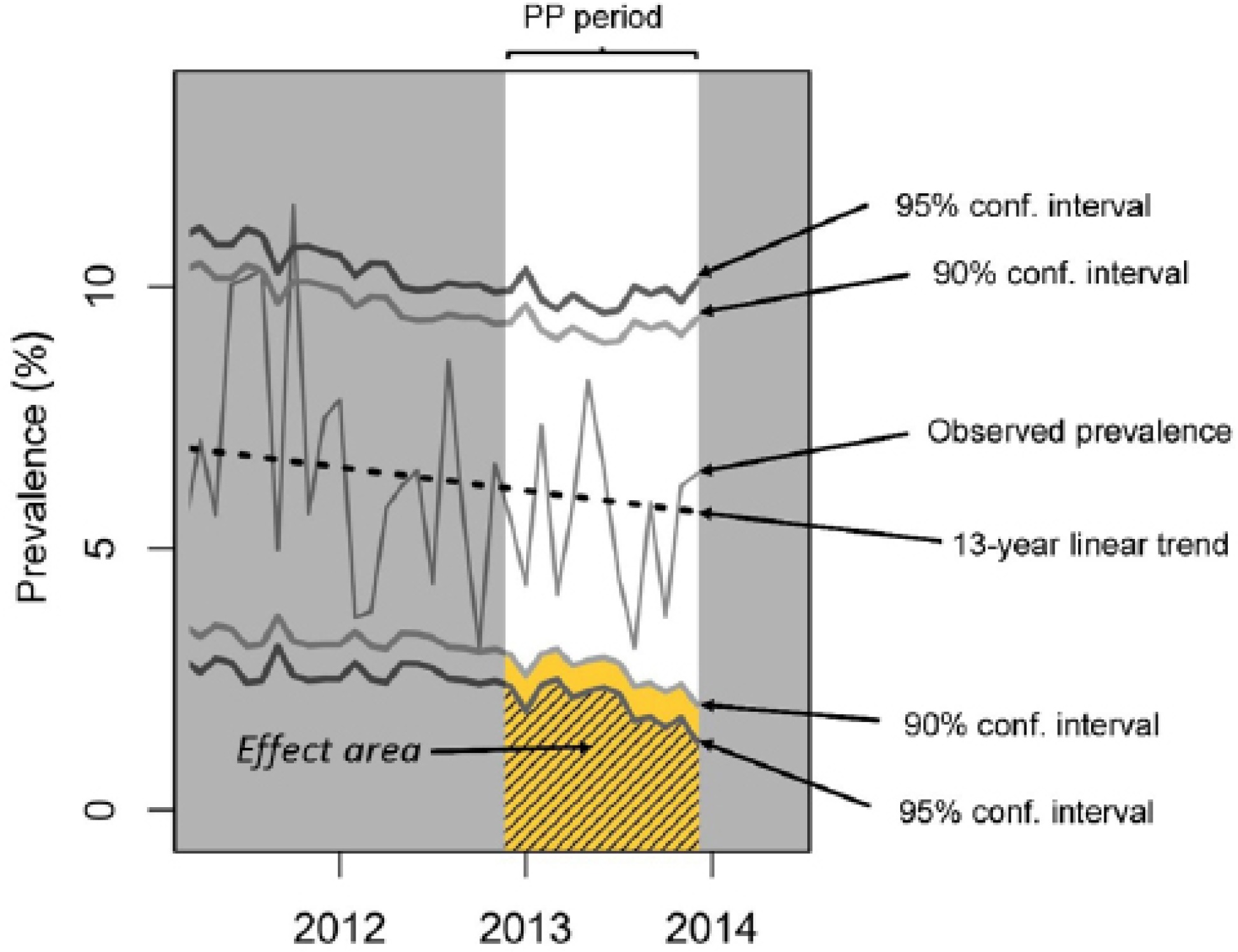
Illustration of Kaul and Wolf’s inference method based on pointwise confidence intervals. If the observed prevalence for any month during the plain packaging period falls in the “effect area”, this is considered as evidence of an effect. Yellow effect area corresponds to confidence intervals at the 90% level of confidence, effect area at the 95% level of confidence.
Power analysis of Kaul and Wolf’s results
In their revised working paper, Kaul and Wolf carried out a formal power analysis to address ‘the concern of whether our trend analysis has any reasonable power at all against a possible plain packaging effect’5. They defined their inference method as consisting of three steps: 1) fitting a linear time-trend using weighted least squares regression, 2) comparing the average of the residuals prior to PP implementation to their average post-PP implementation and carrying out a formal two sample t-test to assess if the post-PP average is smaller than the pre-PP average (if the test rejected the null hypothesis, this was considered as evidence for a PP effect), and finally 3) checking whether any observed prevalence during the PP period was below the 90% pointwise monthly confidence intervals centred at the fitted trend. To help the reader visualize this third step, we call the set of values that are smaller than the fitted trend minus the 90% confidence intervals the effect area20, shown in yellow in Figure 1. Kaul and Wolf interpret any observed monthly prevalence falling in the effect area as evidence of a PP effect. If, instead of 90% confidence intervals, 95% confidence intervals are used, the effect area gets smaller, as illustrated by the hatched area in Figure 1. They computed the estimated power values by Monte-Carlo simulation with ‘generated pseudo prevalence data according a model that is in agreement with the observed data but has a specified plain packaging effect’5. They considered plain packages effects (variable Δ) ranging from 0.25% to 1.5%, in increments of 0.25%, and assumed the effect was ‘enforced’ from December 2012 onwards, i.e. they used the immediate (or sudden) effect model described by Laverty and colleagues13.
For each month t, Kaul and Wolf’s algorithm generated pseudo prevalence values that were distributed according to the normal distribution 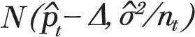
with means  and variance
  where
where  is the prevalence value corresponding to the trend line at month t,
  is the estimated variance of the residuals to the fitted trend line, and nt is the number of observations for month t. There are two issues with the choice of this distribution and its parameters. For simulation to be meaningful, the pseudo data should behave as much as possible like real data. In this case, real data follow a binomial distribution: for each month t = 1,...,156, a random sample of size nt is assumed to be drawn from a large population in which smoking prevalence is pt. The number of smokers in the sample is thus a random variable following the B(nt, pt) binomial distribution. A common rule of thumb is that the normal distribution provides a good approximation of the binomial distribution when pt χnt > 10. However, the first issue is that, with the data at hand, there are many combinations of parameters where this criterion is not met and where, therefore, the normal distribution poorly approximates the underlying distribution. It is therefore preferable to use the binomial distribution to generate pseudo prevalence values. This is easily done in the R statistical programming language by using the rbinom function instead of rnorm function, with no computational penalty.
The second, more significant, issue is that the variance used by Kaul and Wolf,  remains constant for all pt prevalence values, across all months t = 1,…,156, while the binomial variance is a function of pt, i.e. ,
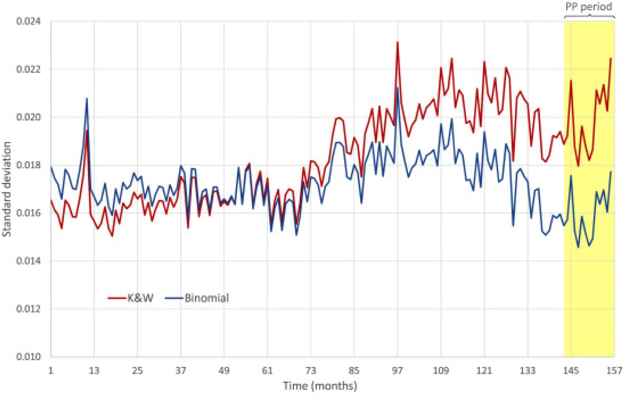
  , and varies each month as pt decreases with time. Figure 2 shows that the standard deviation used by Kaul and Wolf in their power calculation is substantially higher than the standard deviation of the binomial distribution during the PP period, leading the Monte Carlo simulation to more likely generate extreme values and trigger situations that Kaul and Wolf regard as indications of a PP effect, thus artificially inflating the power values of their test.
To remedy this anomaly, we have redone Kaul and Wolf’s power calculations with random data generated with the B(nt,  ) binomial distribution, using the same immediate effect model as they did, as well as the gradual effect model suggested by Laverty and colleagues, ‘in which the potential impact of standardised packaging effect is gradual, increasing linearly to reach the predicted decrease at the end of a given period’13.
In addition to their ‘liberal’ inference method that assumes a PP effect if at least one observed monthly prevalence is below the 90% pointwise confidence interval centred on the fitted trend, Kaul and Wolf envisaged several variations of their methodology, which they called ‘more conservative approaches’5. The first variation they proposed was to change the confidence level from 90% to 95%, which they say is ‘more standard in applied research and would result in wider confidence intervals’. To verify whether such a more conservative method does indeed ‘reinforce’ the authors’ conclusion, as they stated, we have also run the power calculations with pointwise confidence intervals at the 95% level.
All simulations were done with 100,000 Monte Carlo repetitions.
Logistic regression analysis
The logistic regression model for binary data is a robust and more appropriate alternative to multiple linear regression for proportions21. As seen in the previous section, of the prevalence figures contained in the reconstructed Roy Morgan dataset, are derived from the aggregation of individual dichotomous (smoker/non-smoker) variables. We thus fitted a logistic regression model with the number of minors who smoked and the number who did not smoke each month as the outcome variable, using the indicator variables shown below for PP and for other tobacco control measures that may have confounded the potential impact of PP: Each variable comprises 156
values, one for each ordinal month, from month 1 (January 2001) to month 156 (December 2013). Indicator variables take the values 0 (‘not implemented’) or 1 (‘implemented’). The smoke.free variable also contains intermediate values reflecting the proportion of the Australian population living in States with smoke-free policies, as the measure was progressively implemented throughout the country (we refer the reader to Diethelm and Farley14 for a detailed description). The full dataset, including indicator variables, is shown in the supplementary on line material.
We ran stepwise (forward selection, backward elimination, bidirectional selection) logistic regression, selecting the model with smallest Akaike Information Criterion (AIC – a function of the number of parameters fitted and the log likelihood). All analyses were performed with the R statistical programming language.
We also performed a power analysis to check the power achieved with the logistic regression analysis, to assess the impact of the small samples sizes. This was done using the same Monte Carlo simulation described in the previous section, adjusted for logistic regression. At each iteration, a pseudo number of smokers was generated using the binomial random distribution Bnt  ), where the monthly prevalence
 was as predicted by the logistic model, assuming a range of PP effects from 5% to 25% relative reduction in smoking prevalence. The power figure was then calculated as the proportion of Monte Carlo iterations exhibiting a statistically significant PP effect with p-value , when applying the logistic regression analysis described above.
RESULTS
Power analysis of Kaul and Wolf’s results
The results of the power analysis of Kaul and Wolf’s inference method are presented in Table 1. Column 2 shows their power calculations as presented in Table 2 of their working paper5. For each potential effect of plain packaging from a 0.25% to a 1.50% absolute reduction in smoking prevalence simulated, the re-estimated power figures are all substantially lower than Kaul and Wolf’s estimates. Considering, for instance, the row with a PP effect of 0.5% reduction, Kaul and Wolf attributed a power of 0.64 to their inference method to detect such an effect (column 2), while our calculations show it to be only 0.36 (column 3), assuming, as they did, a sudden PP effect, or even 0.29 (column 4) with a gradual PP effect. Corresponding power values, when Kaul and Wolf’s inference method uses 95% confidence intervals (columns 5-7), are all smaller.
Table 2
Fitted logistic regression models. Final model highlighted in bold. AIC = Akaike Information Criterion.
Logistic regression analysis
Smoking prevalence in minors decreased over the 13-year period from a mean of 11.6% in 2001 to 5.6% in 2013, an overall 52% relative decline (Figure 3). The fitted logistic regression model (blue dotted line) showed a significant 5.5% annual reduction in smoking prevalence (95% confidence interval 4.6% to 6.4%) (Table 2). There was a modest, though not statistically significant, impact of plain packaging (Figure 3, solid red line) introduced from November 2012 with a 12.1% relative reduction in smoking prevalence, equivalent to approximately a 2-year decline in prevalence. All three stepwise regression model selection strategies (forward, backward and bidirectional) resulted in the same model with smallest AIC value. The impact of tax increases on smoking prevalence, introduction of comprehensive smoke-free policies, and graphic health warnings, were very limited and not statistically significant in this dataset.
Figure 3
Times series of observed prevalence with fitted logistic regression lines based on selected model and time trend line
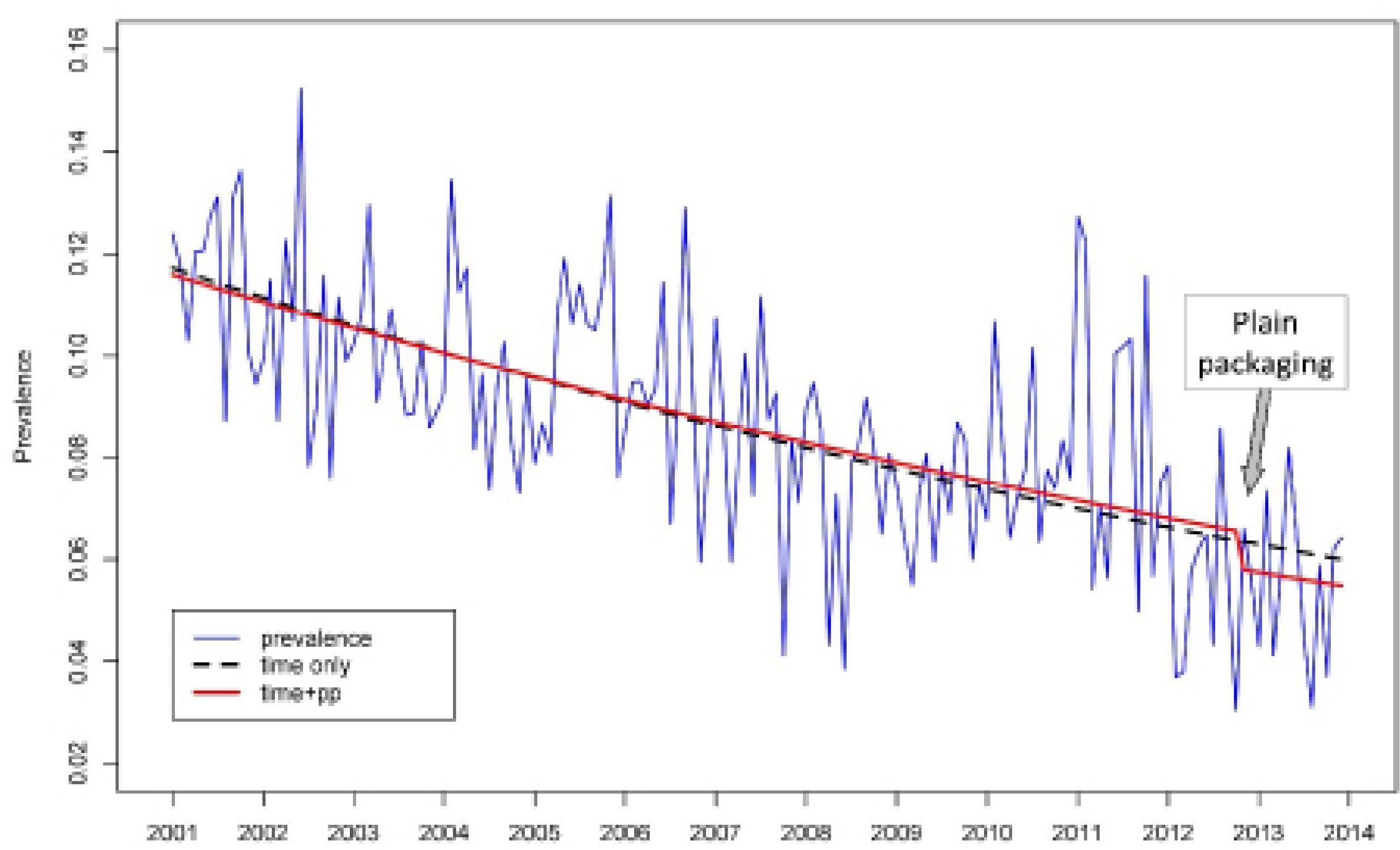
Table 3 shows the power of the logistic regression model to detect (using binomially generated pseudo data) a range of PP effects ranging from 5% to 25% relative reduction, with the estimated PP effect highlighted. The power figures give the probability of finding a statistically significant effect with a p-value 0.05.
Table 3
Power of the logistic regression analysis associated with various plain packaging effects on smoking prevalence (estimated value from fitted model highlighted in bold). Pseudo data were generated using immediate and gradual effect models. Power estimates were obtained with 100,000 Monte Carlo repetitions.
| Reduction in smoking prevalence | Power | |
|---|---|---|
| Immediate effect | Gradual effect | |
| 5% | 0.09 | 0.06 |
| 10% | 0.22 | 0.09 |
| 12.1% | 0.30 | 0.11 |
| 15% | 0.44 | 0.15 |
| 20% | 0.69 | 0.24 |
| 25% | 0.88 | 0.36 |
DISCUSSION
Power analysis of Kaul and Wolf’s results
Our results confirm what Laverty and colleagues11 had pointed out: given the data at hand, and the small sample sizes, Kaul and Wolf’s method lacked sufficient power for detecting the likely impact of PP on smoking prevalence amongst minors in Australia during the first year after the measure was implemented. With the PP effect level that could be plausibly expected (0.5 percentage point absolute decrease of prevalence), their method actually had a much greater probability of not finding an effect than of finding one. It is therefore not surprising that they did not find any evidence of a PP effect. Our results contradict Kaul and Wolf’s statement that ‘if anything’ their analysis was ‘slightly biased in favor of finding a statistically significant (negative) effect of plain packaging on smoking prevalence of Australians aged 14 to 17 years’5. The best that could be said of their analysis is that it was inconclusive.
Furthermore, while emphasizing that their analysis did not discover evidence of a PP effect, Kaul and Wolf added that ‘[m]ore conservative statistical inference methods would only reinforce this conclusion’. Table 1 shows that the power figures, associated with the more ‘conservative’ 95% confidence intervals, are all lower than those associated with their ‘liberal’ 90% counterparts; contrary to their assertion, more conservative approaches are in fact less conclusive. This was to be expected as the effect area associated with 95% confidence intervals (hatched area in Figure 1) is smaller than the effect area associated with 90% confidence intervals.
Logistic regression analysis
The results of the logistic regression analysis show a clear, though not statistically significant, reduction in smoking prevalence following the introduction of plain packaging, equivalent in magnitude to approximately a 2-year relative decline in prevalence. No measurable effect of the other tobacco control measures could be detected in this dataset. This contrasts with a previous analysis14 using identical methods of trends in smoking prevalence among adults, which showed significant reductions in smoking prevalence following a tax increase and the introduction of comprehensive smoke-free policies and plain packaging. However, the dataset on minors is limited compared with that on adults – average sample size 266 compared with 4519, average smoking prevalence 8.6% compared with 21.5% – and it is of little surprise that the impact of different tobacco control measures cannot be detected given the large sampling variation. We note that the introduction of plain packaging was accompanied by a relative reduction in adult smoking prevalence of 3.7%, equivalent in magnitude to approximately a 2-year relative decline in prevalence (1.7%).
Our result concerning the effect of plain packaging on the prevalence of smoking among minors is thus consistent with our result for adults14. It is furthermore consistent with the finding of a recent study22 that provides ‘evidence that a considerable proportion of young smokers tried to quit or thought about quitting as a result of the new Australian tobacco packs in the period following their introduction’.
Power analysis of the logistic regression shows that even if the detected effect was real, there was a low probability of finding a statistically significant result at the p = 0.05 level: only 3 chances out of 10 assuming the PP effect was immediate, or even about 1 out of 10 with a gradual effect, mostly due to the low sample size of the data at hand. Thus, the lack of significance of our result was to be expected and cannot be given any further interpretation.
CONCLUSIONS
On the same day Kaul and Wolf’s first working paper was posted on the website of the University of Zürich, Philip Morris International issued a press release entitled ‘Researchers Find No Evidence Plain Packaging “Experiment” Has Cut Smoking’23, in which the two UZH researchers were quoted explaining: ‘We used statistical methodology that gave every possible leeway for detecting a possible plain packaging effect. Nevertheless, the data does not support any evidence of an actual effect of the Australian Plain Packaging Act on smoking prevalence of minors.’ In the response it submitted a few months later to the UK government’s consultation on standardized packaging24, PMI went even further and presented the results of the UZH study as follows: ‘(…) using standard techniques for statistical analysis and applying the standard statistical significance level of 5%, the experts found no evidence that “standardised packaging” had had an effect on smoking prevalence among Australians aged 14 to 17 years old […]. Kaul and Wolf confirmed that if there had been an effect in reality […], it would have been reflected in the data. According to the study, however, no effect was found’. This strong statement was logically equivalent to saying that Kaul and Wolf’s study had actually proved that plain packaging was not effective.
Our results showed that this conclusion was unjustified: Kaul and Wolf’s results on minors are at best inconclusive. Their method applied to the Roy Morgan survey data on minors lacked power to produce a significant conclusion: the critique by Laverty at al.11 is thus confirmed. Furthermore, Kaul and Wolf were mistaken when they claimed that more ‘conservative’ approaches than their ‘liberal’ method would reinforce their findings: we saw that such approaches are actually weaker.
Contrary to Kaul and Wolf’s conclusions, our logistic regression analysis suggests a plain packaging effect in the expected direction, although this is not statistically significant, the data set on minors being too small and thus lacking the power needed to reach a firmer conclusion.